
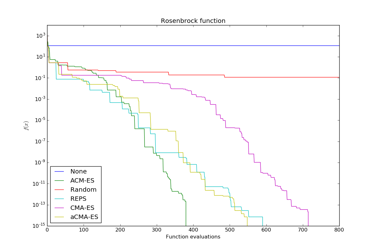
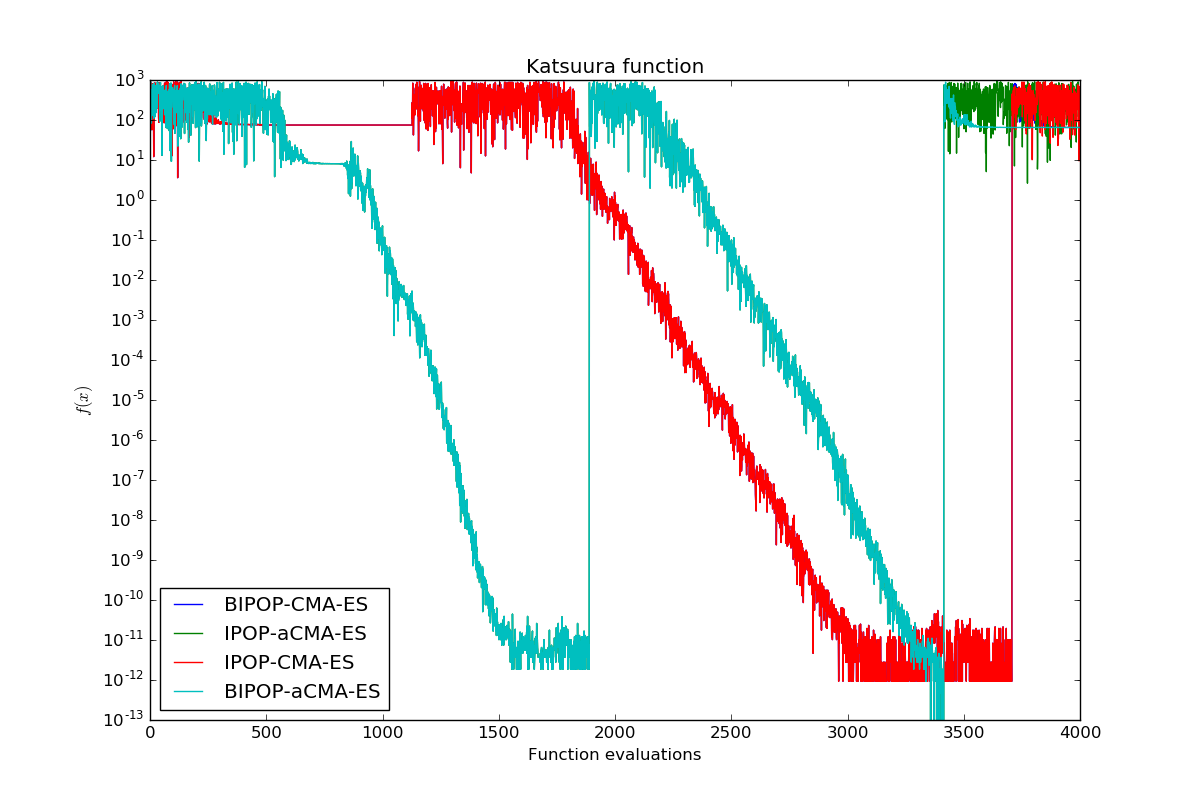
Compare several optimizers for unimodal and multimodal optimization. As a benchmark function for unimodal optimization, the Rosenbrock function will be used. To compare multimodal optimizers, the Katsuura function will be used. Multimodal optimization requires a restart strategy in comparison to unimodal optimization because we might get stuck in a local optimum. Both objective functions will only have two parameters that have to be optimized in this example.
aCMA-ES is a little bit faster than CMA-ES in this example and both are significantly better than random exploration. A very aggressive version of REPS is similarly efficient as aCMA-ES. Another variante of CMA-ES, ACM-ES, outperforms all other optimizers. ACM-ES uses a ranking SVM as a surrogate model.
We compare several multimodal variants of CMA-ES on the Katsuura function. IPOP (increasing population size) and BIPOP (Bi-population) refer to different restart strategy and the “a” (active) indicates another search distribution update. IPOP and BIPOP do not differ very much at the beginning, however, the active update makes a difference in this example.
print(__doc__)

import numpy as np
from bolero.optimizer import (NoOptimizer, RandomOptimizer, CMAESOptimizer,
                              IPOPCMAESOptimizer, BIPOPCMAESOptimizer,
                              REPSOptimizer, ACMESOptimizer)
from bolero.environment.objective_functions import Rosenbrock, Katsuura
import matplotlib.pyplot as plt


def eval_loop(Opt, opt, n_dims, n_iter):
    x = np.empty(n_dims)
    opt.init(n_dims)
    objective = Opt(0, n_dims)
    results = np.empty(n_iter)
    for i in xrange(n_iter):
        opt.get_next_parameters(x)
        results[i] = objective.feedback(x)
        opt.set_evaluation_feedback(results[i])
    return results - objective.f_opt


n_dims = 2
n_iter = 800
x = np.zeros(n_dims)

optimizers = {
    "None": NoOptimizer(x),
    "Random": RandomOptimizer(x, random_state=0),
    "CMA-ES": CMAESOptimizer(x, bounds=np.array([[-5, 5]]), random_state=0),
    "aCMA-ES": CMAESOptimizer(x, bounds=np.array([[-5, 5]]), active=True,
                              random_state=0),
    "REPS": REPSOptimizer(x, random_state=0),
    "ACM-ES": ACMESOptimizer(x, random_state=0)
    }

plt.figure(figsize=(12, 8))
plt.xlabel("Function evaluations")
plt.ylabel("$f(x)$")
plt.title("Rosenbrock function")
for name, opt in optimizers.items():
    r = eval_loop(Rosenbrock, opt, n_dims, n_iter)
    plt.plot(-np.maximum.accumulate(r), label=name)
plt.yscale("log")
plt.legend(loc='best')

n_dims = 2
n_iter = 4000
x = np.zeros(n_dims)

optimizers = {
    "IPOP-CMA-ES": IPOPCMAESOptimizer(x, bounds=np.array([[-5, 5]]),
                                      random_state=0),
    "BIPOP-CMA-ES": BIPOPCMAESOptimizer(x, bounds=np.array([[-5, 5]]),
                                        random_state=0),
    "IPOP-aCMA-ES": IPOPCMAESOptimizer(x, bounds=np.array([[-5, 5]]),
                                       active=True, random_state=0),
    "BIPOP-aCMA-ES": BIPOPCMAESOptimizer(x, bounds=np.array([[-5, 5]]),
                                         active=True, random_state=0),
    }

plt.figure(figsize=(12, 8))
plt.xlabel("Function evaluations")
plt.ylabel("$f(x)$")
plt.title("Katsuura function")
for name, opt in optimizers.items():
    plt.plot(-eval_loop(Katsuura, opt, n_dims, n_iter), label=name)
plt.yscale("log")
plt.legend(loc='best')

plt.show()
Total running time of the script: ( 0 minutes 12.065 seconds)