
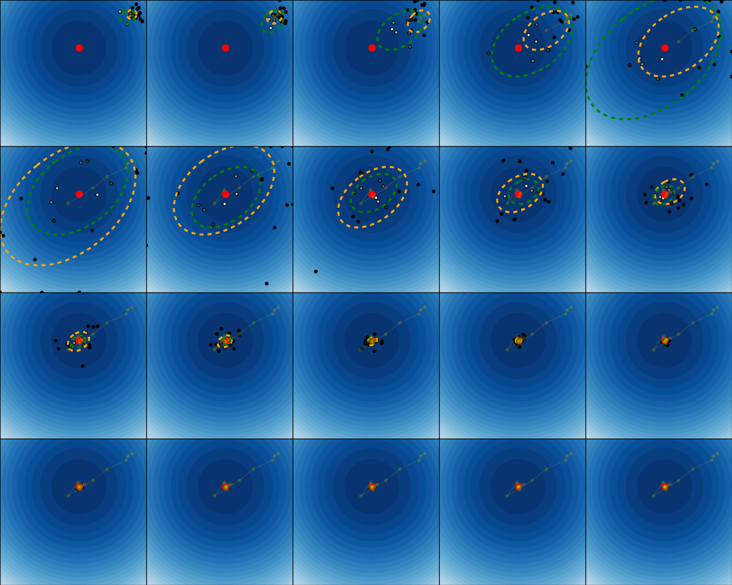
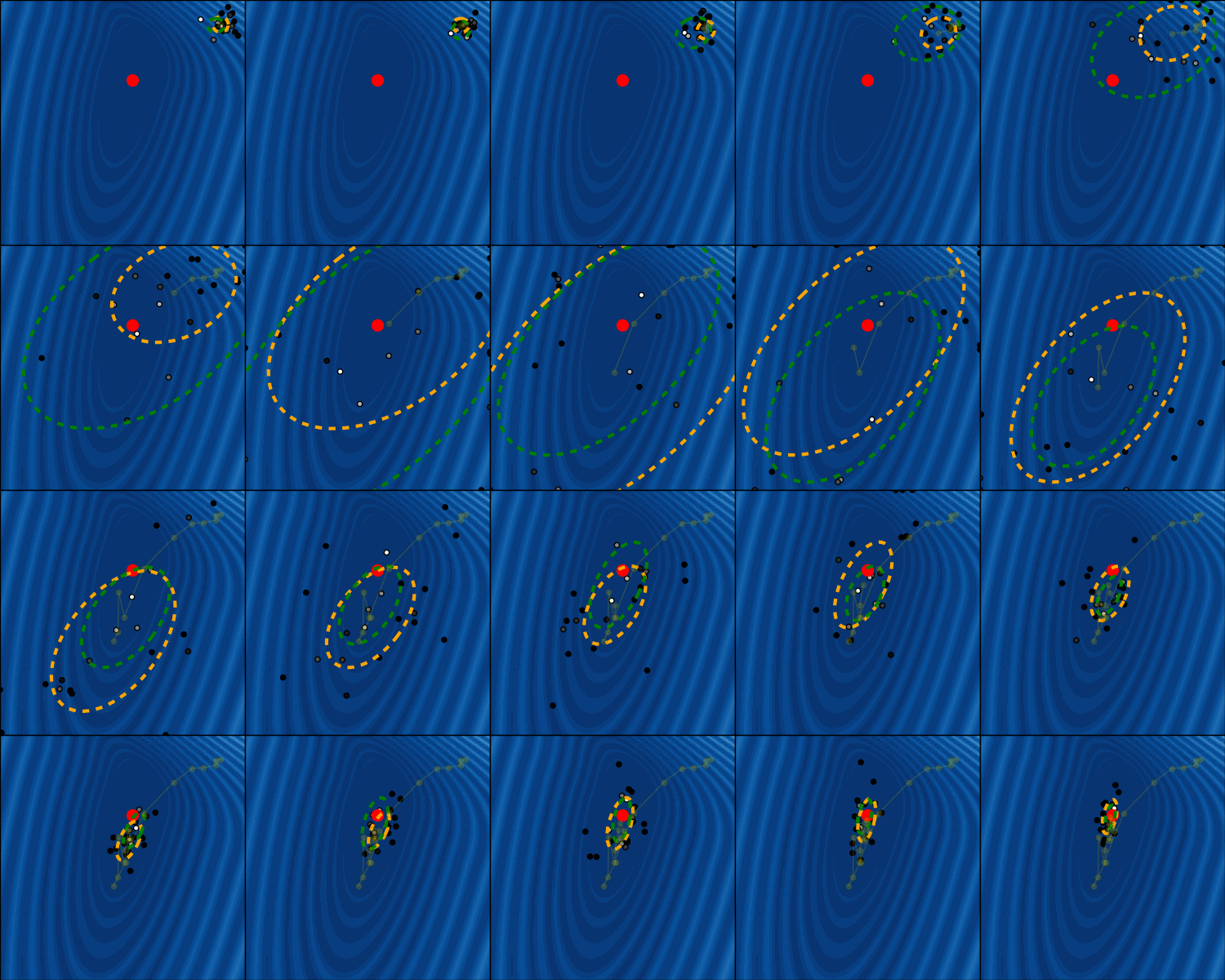
In this example, we see how CMA-ES works by means of two objective functions: it has a Gaussian search distribution (illustrated by the orange equiprobable ellipse) from which samples are drawn.
Each sample is evaluated on the objective function and than weighted by its rank in the current generation (samples with higher weights are whiter). The weighted samples will be used to update the search distribution (covariance and mean) for the next generation (green equiprobable ellipse). The optimum of the objective function is marked with a red dot and the objective function values for the search space are color-coded.
print(__doc__)

import numpy as np
import matplotlib.pyplot as plt
from matplotlib.patches import Ellipse
from bolero.environment.objective_functions import FUNCTIONS
from bolero.optimizer import CMAESOptimizer


def plot_objective():
    x, y = np.meshgrid(np.arange(-6, 6, 0.1), np.arange(-6, 6, 0.1))
    z = np.array([[objective.feedback([y[i, j], x[i, j]])
                   for i in range(x.shape[0])]
                   for j in range(x.shape[1])])
    plt.contourf(x, y, z, cmap=plt.cm.Blues,
                 levels=np.linspace(z.min(), z.max(), 30))
    plt.setp(plt.gca(), xticks=(), yticks=(), xlim=(-5, 5), ylim=(-5, 5))


def equiprobable_ellipse(cov, factor=1.0):
    """Source: http://stackoverflow.com/questions/12301071"""
    def eigsorted(cov):
        vals, vecs = np.linalg.eigh(cov)
        order = vals.argsort()[::-1]
        return vals[order], vecs[:,order]
    vals, vecs = eigsorted(cov)
    angle = np.arctan2(*vecs[:,0][::-1])
    width, height = 2 * factor * np.sqrt(vals)
    return angle, width, height


def plot_ellipse(cov, mean, color):
    angle, width, height = equiprobable_ellipse(cov)
    e = Ellipse(xy=mean, width=width, height=height, angle=np.degrees(angle),
                ec=color, fc="none", lw=3, ls="dashed")
    plt.gca().add_artist(e)


n_generations = 20
n_samples_per_update = 20
n_params = 2


for objective_name in ["Sphere", "SchaffersF7"]:
    objective = FUNCTIONS[objective_name](0, n_params)

    initial_params = 4.0 * np.ones(n_params)
    cmaes = CMAESOptimizer(
        initial_params=initial_params, variance=0.1, active=True,
        n_samples_per_update=n_samples_per_update,
        bounds=np.array([[-5, 5], [-5, 5]]), random_state=0)
    cmaes.init(n_params)

    n_rows = 4
    plt.figure(figsize=(n_generations * 3 / n_rows, 3 * n_rows))
    path = []
    for it in range(n_generations):
        plt.subplot(n_rows, n_generations / n_rows, it + 1)
        plot_objective()
        last_mean = cmaes.mean.copy()
        path.append(last_mean)
        last_cov = cmaes.var * cmaes.cov

        X = np.empty((n_samples_per_update, n_params))
        F = np.empty((n_samples_per_update, 1))
        for i in range(n_samples_per_update):
            cmaes.get_next_parameters(X[i])
            F[i, :] = objective.feedback(X[i])
            cmaes.set_evaluation_feedback(F[i])

        current_path = np.array(path)
        plt.plot(current_path[:, 0], current_path[:, 1], "o-", c="y", alpha=0.2)

        weights = np.zeros(n_samples_per_update)
        weights[np.argsort(F.ravel())[::-1][:len(cmaes.weights)]] = cmaes.weights
        plt.scatter(X[:, 0], X[:, 1], c=weights, cmap=plt.cm.gray)
        plt.scatter(objective.x_opt[0], objective.x_opt[1], s=100, color="r")

        plot_ellipse(cov=last_cov, mean=last_mean, color="orange")
        plot_ellipse(cov=cmaes.var * cmaes.cov, mean=cmaes.mean, color="green")
    plt.subplots_adjust(left=0, bottom=0, right=1, top=1, wspace=0, hspace=0)
plt.show()
Total running time of the script: ( 0 minutes 44.068 seconds)